library(tidyverse)
library(janitor)
library(tidylog)
theme_set(theme_minimal())Data Processing
Overview
Now that the data have been imported and the features renamed, the data can be cleaned and examined to ensure that it is accurate, complete, and consistent.
Feature Inspection
Explore the individual features in the dataset, looking for outliers, bad data points, and unusual or surprising patterns in the data. For categorical features, look for miscoded values or anything else that might interfere with the analysis.
year
We know from the county dashboard that the data should be from 2011 to 2021. This feature is really categorical, not numeric. There is also a distinct order, so it will be converted into an ordinal factor.
df_counties |>
  distinct(year) |> pull()
distinct: removed 7,029 rows (>99%), 11 rows remaining [1] 2011 2012 2013 2014 2015 2016 2017 2018 2019 2020 2021There are 10 distinct year values, which is expected. Given that the data are correct, we can now convert to a factor because year is not really a numeric feature. Instead, it is an ordinal categorical feature.
df_counties <- df_counties |>
  mutate(
    year = fct_inseq(factor(year, ordered = TRUE))
  )
mutate: converted 'year' from double to ordered factor (0 new NA)head(df_counties$year)[1] 2011 2011 2011 2011 2011 2011
11 Levels: 2011 < 2012 < 2013 < 2014 < 2015 < 2016 < 2017 < 2018 < ... < 2021Now year is a factor ordered sequentially.
geography
The geography feature contains the state and county names. There are 39 counties in Washington, so we expect that there will be 40 distinct values in this feature. This feature is also categorical in nature, but nominal rather than ordinal.
df_counties |>
  distinct(geography) |> pull()
distinct: removed 7,000 rows (99%), 40 rows remaining [1] "Washington State" "Yakima" "Whitman" "Whatcom"
[5] "Walla Walla" "Wahkiakum" "Thurston" "Stevens"
[9] "Spokane" "Snohomish" "Skamania" "Skagit"
[13] "San Juan" "Pierce" "Pend Oreille" "Pacific"
[17] "Okanogan" "Mason" "Lincoln" "Lewis"
[21] "Klickitat" "Kittitas" "Kitsap" "King"
[25] "Jefferson" "Island" "Grays Harbor" "Grant"
[29] "Garfield" "Franklin" "Ferry" "Douglas"
[33] "Cowlitz" "Columbia" "Clark" "Clallam"
[37] "Chelan" "Benton" "Asotin" "Adams" It looks like the data are correct. There are 40 distinct values, as expected.
df_counties <- df_counties |>
  mutate(
    geography = factor(geography)
  )
mutate: converted 'geography' from character to factor (0 new NA)levels(df_counties$geography) [1] "Adams" "Asotin" "Benton" "Chelan"
[5] "Clallam" "Clark" "Columbia" "Cowlitz"
[9] "Douglas" "Ferry" "Franklin" "Garfield"
[13] "Grant" "Grays Harbor" "Island" "Jefferson"
[17] "King" "Kitsap" "Kittitas" "Klickitat"
[21] "Lewis" "Lincoln" "Mason" "Okanogan"
[25] "Pacific" "Pend Oreille" "Pierce" "San Juan"
[29] "Skagit" "Skamania" "Snohomish" "Spokane"
[33] "Stevens" "Thurston" "Wahkiakum" "Walla Walla"
[37] "Washington State" "Whatcom" "Whitman" "Yakima" The levels have been recorded alphabetically, which makes sense for the most part. Since “Washington State” isn’t a county, it can be repositioned at the front, to separate it from the counties.
df_counties$geography <- fct_relevel(df_counties$geography, "Washington State", after=0)
levels(df_counties$geography)
[1] "Washington State" "Adams" "Asotin" "Benton"
[5] "Chelan" "Clallam" "Clark" "Columbia"
[9] "Cowlitz" "Douglas" "Ferry" "Franklin"
[13] "Garfield" "Grant" "Grays Harbor" "Island"
[17] "Jefferson" "King" "Kitsap" "Kittitas"
[21] "Klickitat" "Lewis" "Lincoln" "Mason"
[25] "Okanogan" "Pacific" "Pend Oreille" "Pierce"
[29] "San Juan" "Skagit" "Skamania" "Snohomish"
[33] "Spokane" "Stevens" "Thurston" "Wahkiakum"
[37] "Walla Walla" "Whatcom" "Whitman" "Yakima" Now the factor is set up properly.
selection_filter
selection_filter should be a categorical feature. First, determine what the set of possible values is.
df_counties |>
  distinct(selection_filter) |> pull()
distinct: removed 7,036 rows (>99%), 4 rows remaining[1] "All" "Sex" "Age" "Race/Ethnicity"These are all reasonable. The only one that we are interested in is the Age filter so we will only keep observations from the dataset with Age as the selection_filter value.
df_counties <- df_counties |>
  filter(selection_filter == "Age")
filter: removed 4,400 rows (62%), 2,640 rows remainingselection_value
The selection values should now only pertain to Age.
df_counties |>
  distinct(selection_value) |> pull()
distinct: removed 2,634 rows (>99%), 6 rows remaining[1] "65+" "45-64" "25-44" "15-24" "1-14" "<1" These values look correct. Nothing more needs to be done with this variable.
max_percent_total_population
This feature pertains to what percentage of the population a given filter applies to for the given geography. It’s a percentage, so all values should be between 0 and 100.
summary(df_counties$max_percent_total_population) Min. 1st Qu. Median Mean 3rd Qu. Max.
0.4691 11.1973 16.9423 16.6667 24.2378 43.3292 There are no missing values and all values are positive and range between 0 and 100, so this data is valid.
max_sub_population
This feature pertains to the number of people that fall into the given selection_filter/selection_value combination for the given geography. All values should be positive and no larger than the total population of the state (at most).
summary(df_counties$max_sub_population) Min. 1st Qu. Median Mean 3rd Qu. Max.
12.7 2112.5 9173.4 60373.6 25492.6 2190675.0 This is the case. There are no missing values.
max_total_population
Without a codebook, it is not clear what this feature represents. Furthermore, most of the observations are missing data for this variable. Given that this field won’t be required for our purposes, it will be removed from the dataset.
summary(df_counties$max_total_population) Min. 1st Qu. Median Mean 3rd Qu. Max. NA's
2286 17835 45835 70978 86918 542100 2232 df_counties <- df_counties |>
select(-max_total_population)select: dropped one variable (max_total_population)Dataframe pivot and new feature creation
Now, we need to pivot all of the age data into a single observation so that we can perform different dependency ratio calculations for each year/geography combination. We will need to first filter out all of the non Age selection filters, then drop the variables that we don’t need for our calculations so that we get a single observation for each year/geography combination.
df_counties <- df_counties |>
  select(-c(max_percent_total_population, selection_filter)) |>
  pivot_wider(names_from=selection_value, values_from=max_sub_population, names_prefix="age_") |>
  clean_names()
select: dropped 2 variables (selection_filter, max_percent_total_population)pivot_wider: reorganized (selection_value, max_sub_population) into (age_65+, age_45-64, age_25-44, age_15-24, age_1-14, …) [was 2640x4, now 440x8]df_counties <- df_counties |>
mutate(
total_dep_ratio = round((age_65 + age_1_14 + age_1)/(age_45_64 + age_25_44 + age_15_24)*100,2),
child_dep_ratio = round((age_1_14 + age_1)/(age_45_64 + age_25_44 + age_15_24)*100,2),
aged_dep_ratio = round((age_65)/(age_45_64 + age_25_44 + age_15_24)*100,2)
)mutate: new variable 'total_dep_ratio' (double) with 415 unique values and 0% NA new variable 'child_dep_ratio' (double) with 371 unique values and 0% NA new variable 'aged_dep_ratio' (double) with 418 unique values and 0% NAUnivariate checks on new features
Now that new dependency ratio features have been created, they need to be checked to ensure that the values are reasonable. tidylog output indicates that there are no NA values in the new features. We now need to plot data to ensure that the values are reasonable.
total_dep_ratio
The total dependency ratio should be positive. A histogram, faceted by year shows that the values for all years are plausible. There are no negative values and the distributions do not show any extreme outliers.
df_counties |>
  ggplot(aes(x=total_dep_ratio)) +
  geom_histogram(colour="white") +
  labs(
    x="Total dependency ratio",
    y="Count",
    title="Total dependency ratio distrution"
  ) +
  facet_wrap(~year)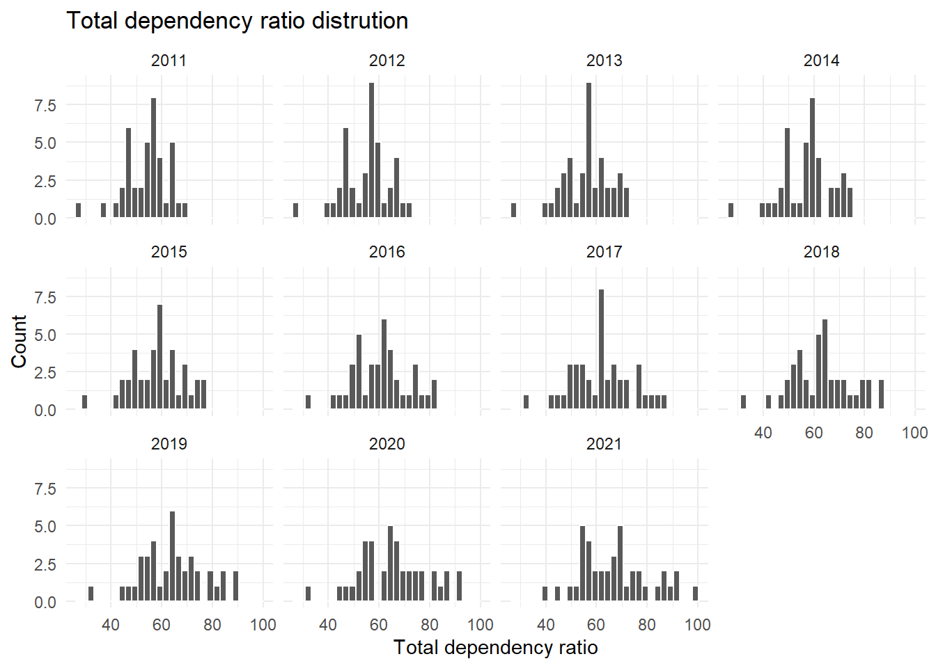
child_dep_ratio
The child dependency ratio should always be positive. A histogram, faceted by year shows that the values for all years are plausible. There are no negative values and the distributions do not show any extreme outliers.
df_counties |>
  ggplot(aes(x=child_dep_ratio)) +
  geom_histogram(colour="white") +
  labs(
    x="Child dependency ratio",
    y="Count",
    title="Child dependency ratio distrution"
  ) +
  facet_wrap(~year)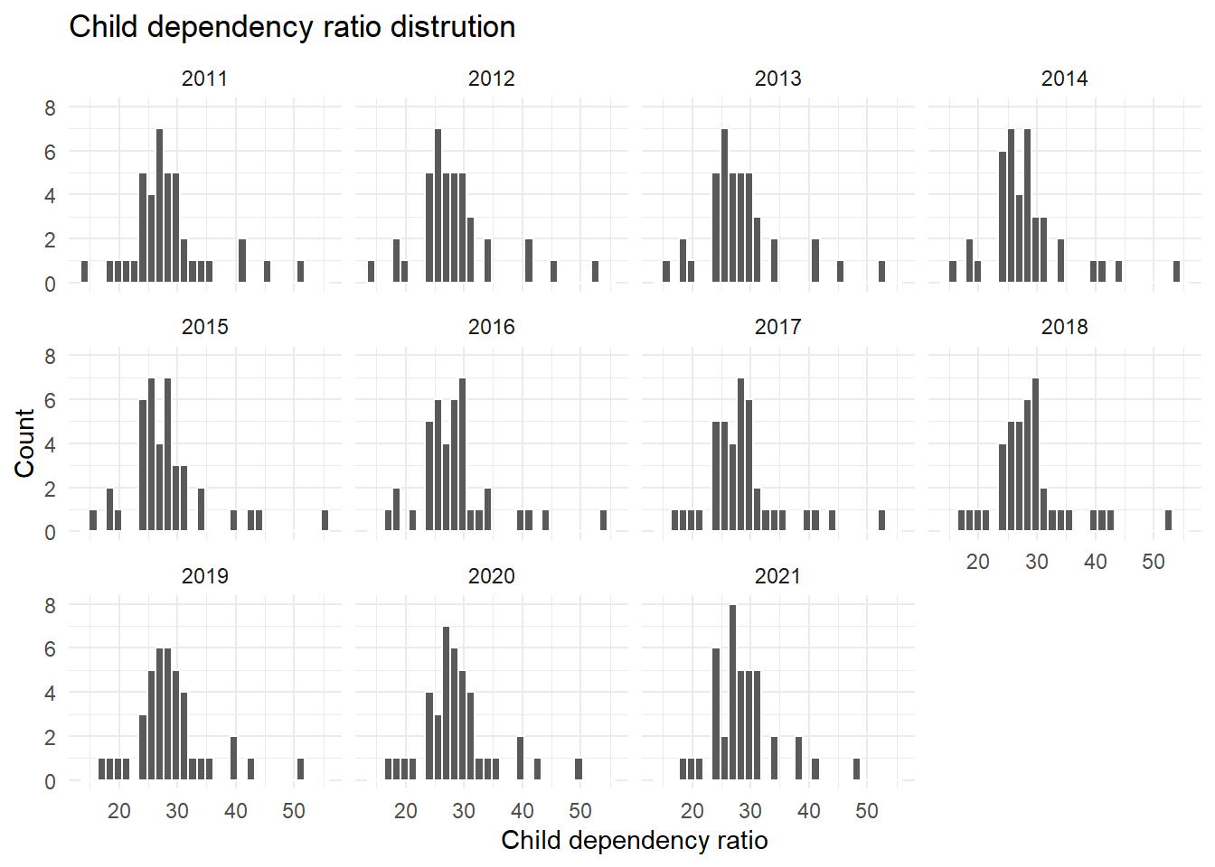
aged_dep_ratio
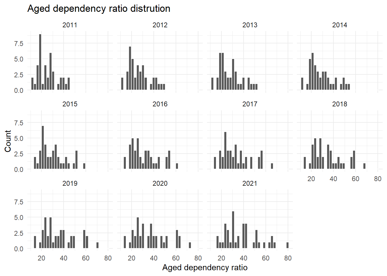
The aged dependency ratio should always be positive. A histogram, faceted by year shows that the values for all years are plausible. There are no negative values and the distributions do not show any extreme outliers.
df_counties |>
  ggplot(aes(x=aged_dep_ratio)) +
  geom_histogram(colour="white") +
  labs(
    x="Aged dependency ratio",
    y="Count",
    title="Aged dependency ratio distrution"
  ) +
  facet_wrap(~year)