Robbery Hotspots in East Denver, 2021

Overview

The analysis looks at robberies in Denver in 2021. The initial focus is on the entire city and observations that can be made about the city in general, but then focuses on 7 neighborhoods in east Denver. After assessing the density of robberies in these neighborhoods, the proximity of robbery hot spots to Regional Transportation District - Denver (RTD) bus stops is considered. Recommendations to RTD planners on where to allocate anti-crime resources are made in the conclusion.

Inital set up

To being, neighborhood boundaries and robbery point data are imported and transformed. The kernel density of robberies is computed and then the density plot is clipped to the neighborhood boundaries so that no density information is displayed for areas where we do not have data.

Code

nbhds <- st_read("geometry/Denver-Statistical-Neighborhoods.geojson", quiet = TRUE) |> 
  st_transform("EPSG:2232")

nbhd_bbox <- st_bbox(nbhds)

# We are only looking at 2021 data
df_robbery_sf <- transform_filter(df_robbery, nbhd_bbox)

# generate the kernel density grid
df_robbery_kde <- df_robbery_sf |> 
  # Calculate density
  hotspot_kde(bandwidth_adjust = 0.5, quiet = TRUE) |> 
  # Clip the density layer to the area for which we have data
  st_intersection(nbhds)

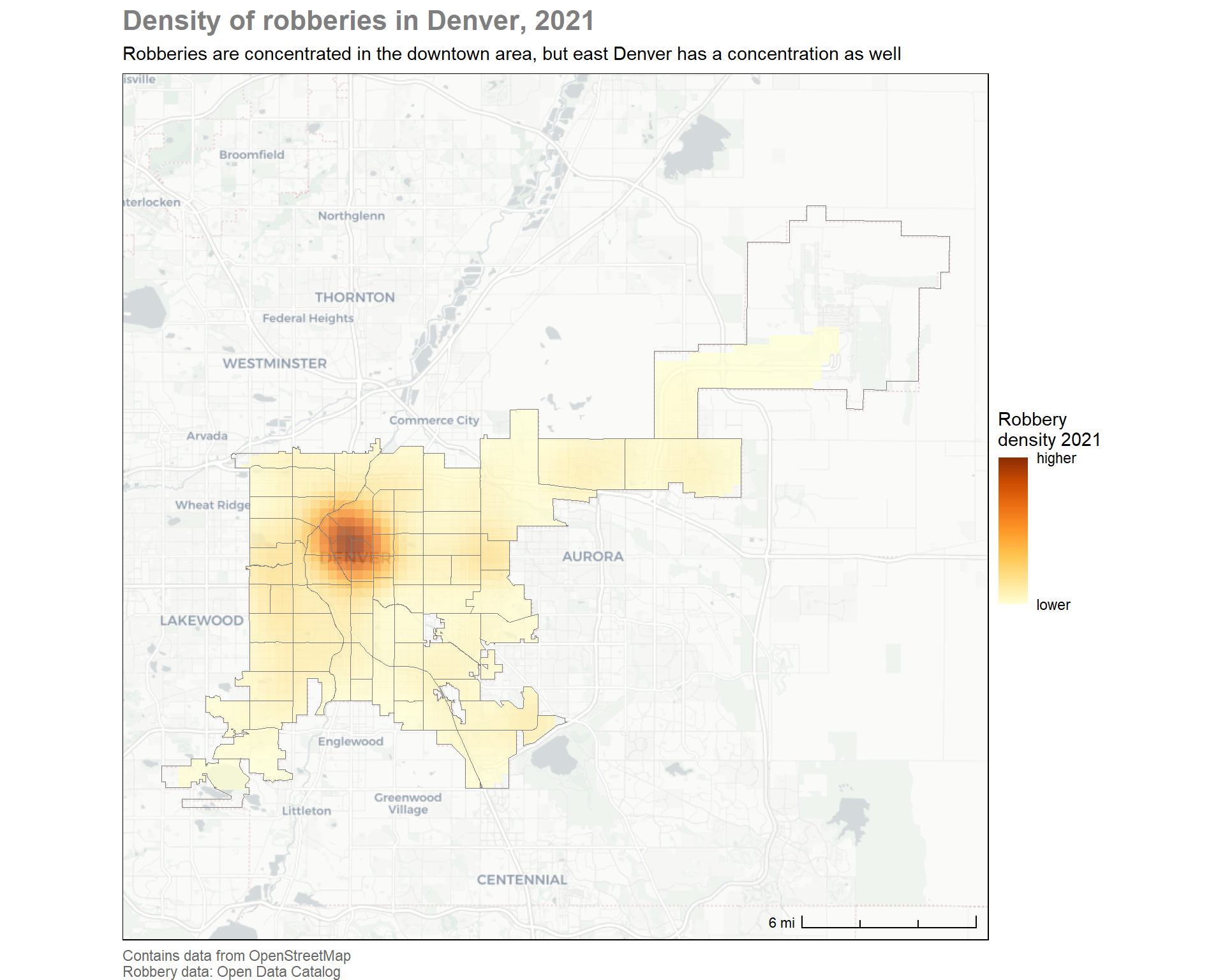
The following density map shows robbery density for the city of Denver in 2021. Robbery activity is clearly concentrated in a few neighborhoods in the downtown area. There appears to be more widely spread, diffuse pattern of robberies across the western half of the city and a notable area of increased density centered in the East Colfax neighborhood in east Denver. The seven neighborhoods in the vicinity of East Colfax will be the focus of this analysis.

Code

ggplot() + 
  # Use openstreet map for a background map.
  annotation_map_tile(type = "cartolight", zoomin = 0, progress = "none") +
  geom_sf(
    aes(fill = kde), 
    data = df_robbery_kde, 
    alpha = 0.75, 
    colour = NA
  ) +
  scale_fill_distiller(
    palette = "YlOrBr",
    direction=1, 
    breaks = range(pull(df_robbery_kde, kde)), 
    labels = c("lower", "higher")
  ) +
  geom_sf(data=nbhds, colour="grey50", fill=NA) +
  annotation_scale(style="ticks", location="br", unit_category="imperial") +
  labs(
    title = "Density of robberies in Denver, 2021",
    subtitle = "Robberies are concentrated in the downtown area, but east Denver has a concentration as well",
    fill = "Robbery\ndensity 2021",
    caption = disclaimer
  ) +
  fixed_plot_aspect()

Robberies in 7 east Denver neighborhoods in 2021

This analysis focuses primarily on y neighborhoods in east Denver: East Colfax, Lowry Field, Montclair, North Park Hill, Northeast Park Hill, South Park Hill, and Stapleton. To narrow our focus down to these 7 neighborhoods, new geometries need to be computed and only robberies occurring in these 7 neighborhoods will be included in the analysis. A new kernel density map will be created from this more narrowly focused dataset.

Code

nbhds_focused <- nbhds |> 
   filter(nbhd_name %in% c(
     "South Park Hill", "East Colfax", "Lowry Field", "Montclair", 
     "Northeast Park Hill", "North Park Hill", "Stapleton"))

nbhd_bbox <- st_bbox(nbhds_focused)

df_robbery_focused_sf <- transform_filter(df_robbery, nbhd_bbox)

# generate the kernel density grid
df_robbery_focused_kde <- df_robbery_focused_sf |> 
  st_intersection(nbhds_focused) |> 
  # Calculate density
  hotspot_kde(
    grid = hotspot_grid(nbhds_focused, cell_size = 100),
    bandwidth_adjust = 0.5, quiet = TRUE
  ) |> 
  # Clip the density layer to the area for which we have data
  st_intersection(nbhds_focused)

Bus stop data

Assessing the risk of robbery at RTD bus stops is achieved by superimposing bus stop locations on the robbery density map. The bus stop location data comes from the OpenStreenMap initiative. Bus stop data is restricted to the neighborhoods of interest after some basic processing is done to fetch the data, restrict it to the bounding box that contains the neighborhoods, and bus stops represented by polygons are collapsed to points. Finally, the coordinate reference system is changed to EPSG:2232 to allow the bus stops to be plotted with the other data.

Code

bus_stops <- nbhds_focused |> 
  st_transform("WGS84") |> 
  st_bbox() |> 
  opq() |> 
  # Define the features we want
  add_osm_feature(key = "highway", value = "bus_stop") |> 
  # Download those features for that area
  osmdata_sf()

# Extract bus stop locations as points
bus_stop_points <- bind_rows(
  pluck(bus_stops, "osm_points"), 
  st_centroid(pluck(bus_stops, "osm_polygons"))
) |> 
  st_intersection(nbhds_focused |> st_transform("WGS84")) |> 
  st_transform("EPSG:2232")

Robbery density in east Denver

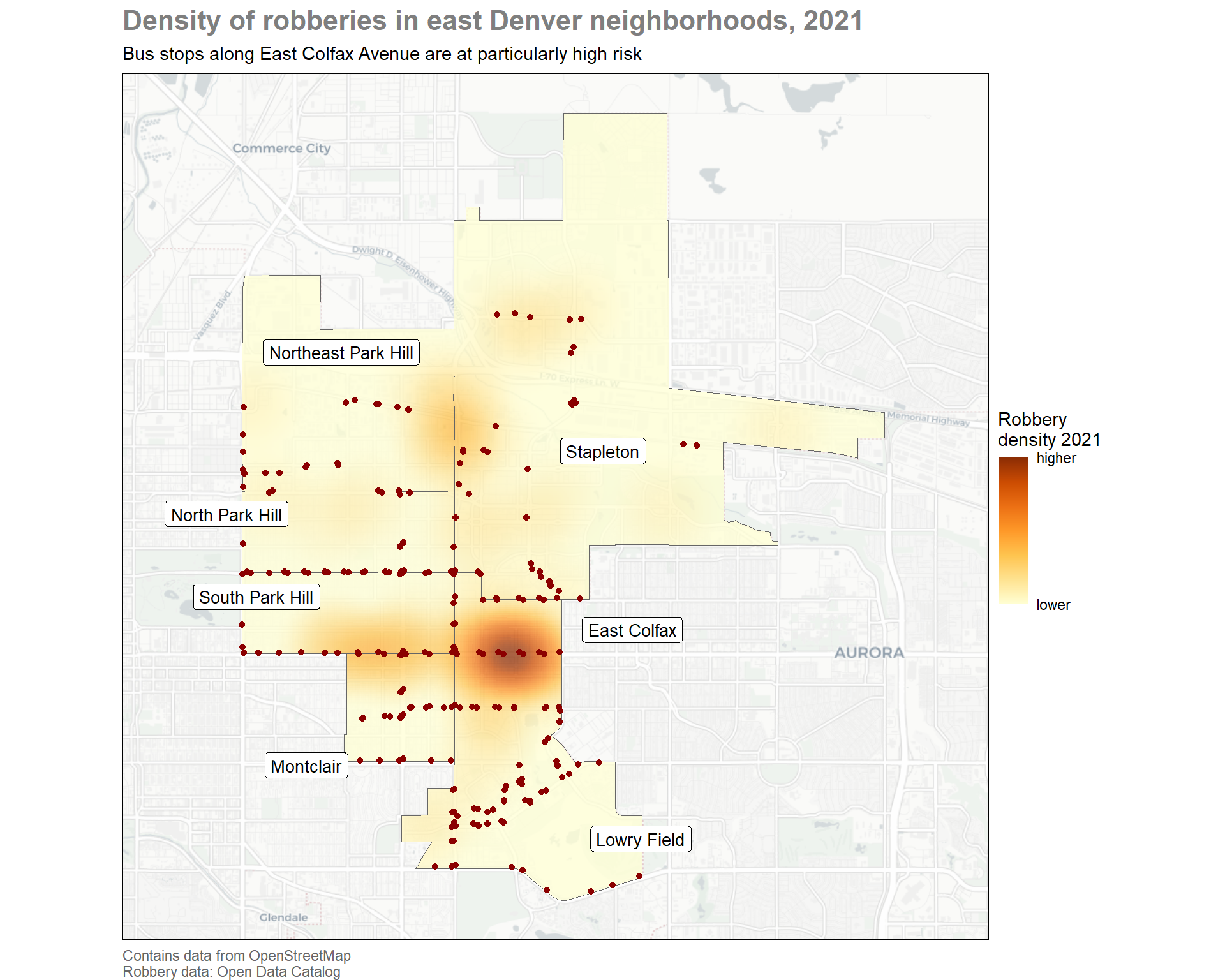
The density map shown below indicates a few important points. First, most robbery crime occurs on East Colfax Avenue with the high density being in the East Colfax neighborhood itself. The map also indicates that there may be another hot spot north of Colfax Avenue on Quebec Street south of I-70. There are a few other potential areas, but it is unclear whether they are statistically significant or not. We will use the Getis-Ord Gi* statistic to identify hot spots in the 7 neighborhoods. Second, it does not appear that bus stops are not generally in areas with high numbers of robberies. It does not appear that bus stops are being specifically targeted in these nieghborhoods. However, the bus stops along Colfax Avenue are located in an area associated with more robberies.

Code

label_size <- 3.5

label_points <- read_csv("geometry/label_points.csv") |> 
  st_as_sf(coords = c("x", "y"),
             crs = "EPSG:2232")
  
ggplot() +
  annotation_map_tile(type = "cartolight", zoomin = 0, progress = "none") +
  geom_sf(aes(fill=kde), data = df_robbery_focused_kde, alpha=0.75, colour = NA) +
  scale_fill_distiller(
    palette = "YlOrBr",
    direction=1,
    breaks = range(pull(df_robbery_focused_kde, kde)),
    labels = c("lower", "higher")
  ) +
  geom_sf(data = nbhds_focused, colour = "grey40", fill = NA) +
  geom_sf(data = bus_stop_points, colour = "darkred") +
  geom_sf_label(data = label_points, aes(label = nbhd_name, geometry = geometry),
                stat = "sf_coordinates", size = label_size) +
  labs(
    title = "Density of robberies in east Denver neighborhoods, 2021",
    subtitle = "Bus stops along East Colfax Avenue are at particularly high risk",
    caption = disclaimer,
    fill = "Robbery\ndensity 2021"
  ) +
  fixed_plot_aspect()

Robbery hot spots and proximity to bus stops

The density map is suggestive of hot spots, but in order to increase our confidence that the hot spots are real, we will use the Gi* statistic to identify areas that have a number of robberies that is not consistent with random chance.

Why a statistic test is important

Policing resources are almost always scarce. Because crime patterns fluctuate over time, there is an element of randomness to the data. A statistical test that can quantitatively identify areas that truly have a high number of crimes that would occur by chance allows planners to allocate scarce resources more efficiently and effectively.

We will compute the Gi* statistic for the 7 neighborhoods using a cell size of 500 feet. As usual, the cells will be clipped to the neighborhoods so that we do not compute hot spot statistics outside of the neighborhoods.

Code

# generate the kernel density grid
df_robbery_focused_gistar <- df_robbery_focused_sf |> 
  st_intersection(nbhds_focused) |> 
  # Calculate density
  hotspot_gistar( 
    grid = hotspot_grid(nbhds_focused, cell_size = 500),
    quiet = TRUE
  ) |> 
  # Clip the density layer to the area for which we have data
  st_intersection(nbhds_focused)

The Gi* statistics computed by the hotspot_gistar function from the sfhotspot package provides a p-value in addition to the value of the statistic. We will filter the results to include only cells that are significant at a significance level of $\alpha = 0.05$ and that have positive values. Negative values indicate areas that have fewer robberies than would be expected by chance.

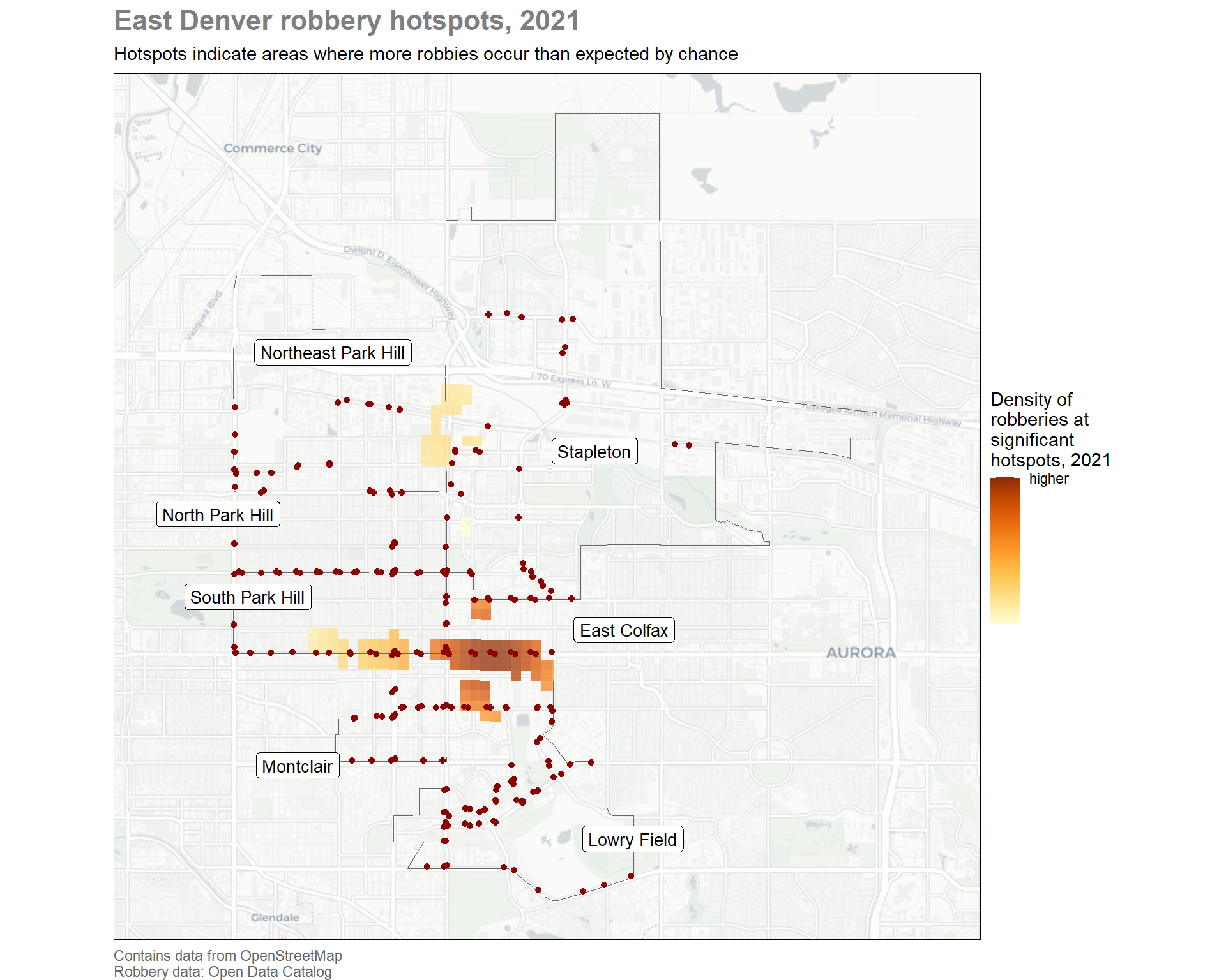
The hot spot map below shows the areas with statistically significant number of robberies. They broadly correspond to the density map shown earlier. East Colfax Avenue is, as expected, the epicenter for robberies in east Denver. One notable departure is that the area in north Stapleton along E 56th Avenue is not a statistical hot spot. The hot spot along Quebec Street is in close proximity to bus stops on its southern edge. Planners way wish to allocate robbery prevention measures at these bus stops.

Code

ggplot() +
  annotation_map_tile(type = "cartolight", zoomin = 0, progress = "none") +
  geom_sf(
    aes(fill = kde),
    data = filter(df_robbery_focused_gistar, gistar > 0, pvalue < 0.05), 
    alpha = 0.75,
    colour = NA
  ) +
  geom_sf(data = nbhds_focused, colour = "grey40", fill = NA) +
  geom_sf(data = bus_stop_points, colour = "darkred") +
  geom_sf_label(data = label_points, aes(label = nbhd_name, geometry = geometry),
                stat = "sf_coordinates", size = label_size) +
  scale_fill_distiller(
    palette = "YlOrBr",
    direction = 1,
    breaks = c(0.01, max(pull(df_robbery_focused_gistar, kde))), 
    labels = c("lower", "higher")
  ) + 
  fixed_plot_aspect() +
  labs(
    title = "East Denver robbery hotspots, 2021",
    subtitle = "Hotspots indicate areas where more robbies occur than expected by chance",
    fill = str_wrap("Density of robberies at significant hotspots, 2021", 15),
    caption = disclaimer
  )

Conclusions and recommendations

Bu stops in east Denver are not systematically associated with increased robbery activity. There are 4 significant robbery hot spots in the 7 neighborhoods, impacting 5 of the 7 neighborhoods. These 4 hot spots should be the primary focus of anti-crime efforts in east Denver. The close proximity of these hot spots may allow for some synergy in efforts to curb robberies and increase awareness of the risk in and around these hot spots. The final hot spot, along Quebec street south of I-70 should also be considered by RTD planners. The cluster of bus stops along the southern boundary of this would be the obvious area to focus resources on.

--- title: "Robbery Hotspots in East Denver, 2021" --- ```{r setup} #| message: false #| echo: false rm(list=ls()) library(tidyverse) library(sf) library(sfhotspot) library(ggspatial) library(osmdata) page_theme <- theme_void() + theme( panel.border = element_rect(colour = "black", fill = NA), plot.caption = element_text(colour = "grey40", hjust = 0), plot.subtitle = element_text(margin = margin(t = 6, b = 6)), plot.title = element_text(colour = "grey50", face = "bold", size = 16) ) theme_set(page_theme) disclaimer <- str_glue( "Contains data from OpenStreetMap", "Robbery data: Open Data Catalog", .sep = "\n" ) # read in the data from intermediates directory df_robbery <- read_rds("intermediates/robbery.rds") transform_filter <- function(data,bbox) { data |> filter(c_year == 2021 & between(geo_x, bbox["xmin"], bbox["xmax"]) & between(geo_y, bbox["ymin"], bbox["ymax"])) |> st_as_sf(coords = c("geo_x", "geo_y"), crs = "EPSG:2232") } ``` ## Overview The analysis looks at robberies in Denver in 2021. The initial focus is on the entire city and observations that can be made about the city in general, but then focuses on 7 neighborhoods in east Denver. After assessing the density of robberies in these neighborhoods, the proximity of robbery hot spots to Regional Transportation District - Denver (RTD) bus stops is considered. Recommendations to RTD planners on where to allocate anti-crime resources are made in the conclusion. ## Inital set up To being, neighborhood boundaries and robbery point data are imported and transformed. The kernel density of robberies is computed and then the density plot is clipped to the neighborhood boundaries so that no density information is displayed for areas where we do not have data. ```{r create simple features objects for the robbery data and neighborhoods} #| warning: false nbhds <- st_read("geometry/Denver-Statistical-Neighborhoods.geojson", quiet = TRUE) |> st_transform("EPSG:2232") nbhd_bbox <- st_bbox(nbhds) # We are only looking at 2021 data df_robbery_sf <- transform_filter(df_robbery, nbhd_bbox) # generate the kernel density grid df_robbery_kde <- df_robbery_sf |> # Calculate density hotspot_kde(bandwidth_adjust = 0.5, quiet = TRUE) |> # Clip the density layer to the area for which we have data st_intersection(nbhds) ``` The following density map shows robbery density for the city of Denver in 2021. Robbery activity is clearly concentrated in a few neighborhoods in the downtown area. There appears to be more widely spread, diffuse pattern of robberies across the western half of the city and a notable area of increased density centered in the East Colfax neighborhood in east Denver. The seven neighborhoods in the vicinity of East Colfax will be the focus of this analysis. ```{r initial 2021 robbery dentist map} #| fig-width: 10 #| fig-height: 8 ggplot() + # Use openstreet map for a background map. annotation_map_tile(type = "cartolight", zoomin = 0, progress = "none") + geom_sf( aes(fill = kde), data = df_robbery_kde, alpha = 0.75, colour = NA ) + scale_fill_distiller( palette = "YlOrBr", direction=1, breaks = range(pull(df_robbery_kde, kde)), labels = c("lower", "higher") ) + geom_sf(data=nbhds, colour="grey50", fill=NA) + annotation_scale(style="ticks", location="br", unit_category="imperial") + labs( title = "Density of robberies in Denver, 2021", subtitle = "Robberies are concentrated in the downtown area, but east Denver has a concentration as well", fill = "Robbery\ndensity 2021", caption = disclaimer ) + fixed_plot_aspect() ``` ## Robberies in 7 east Denver neighborhoods in 2021 This analysis focuses primarily on y neighborhoods in east Denver: East Colfax, Lowry Field, Montclair, North Park Hill, Northeast Park Hill, South Park Hill, and Stapleton. To narrow our focus down to these 7 neighborhoods, new geometries need to be computed and only robberies occurring in these 7 neighborhoods will be included in the analysis. A new kernel density map will be created from this more narrowly focused dataset. ```{r get focused neighborhood data} #| warning: false nbhds_focused <- nbhds |> filter(nbhd_name %in% c( "South Park Hill", "East Colfax", "Lowry Field", "Montclair", "Northeast Park Hill", "North Park Hill", "Stapleton")) nbhd_bbox <- st_bbox(nbhds_focused) df_robbery_focused_sf <- transform_filter(df_robbery, nbhd_bbox) # generate the kernel density grid df_robbery_focused_kde <- df_robbery_focused_sf |> st_intersection(nbhds_focused) |> # Calculate density hotspot_kde( grid = hotspot_grid(nbhds_focused, cell_size = 100), bandwidth_adjust = 0.5, quiet = TRUE ) |> # Clip the density layer to the area for which we have data st_intersection(nbhds_focused) ``` ### Bus stop data Assessing the risk of robbery at RTD bus stops is achieved by superimposing bus stop locations on the robbery density map. The bus stop location data comes from the OpenStreenMap initiative. Bus stop data is restricted to the neighborhoods of interest after some basic processing is done to fetch the data, restrict it to the bounding box that contains the neighborhoods, and bus stops represented by polygons are collapsed to points. Finally, the coordinate reference system is changed to `EPSG:2232` to allow the bus stops to be plotted with the other data. ```{r get OSM bus stop data} #| warning: false bus_stops <- nbhds_focused |> st_transform("WGS84") |> st_bbox() |> opq() |> # Define the features we want add_osm_feature(key = "highway", value = "bus_stop") |> # Download those features for that area osmdata_sf() # Extract bus stop locations as points bus_stop_points <- bind_rows( pluck(bus_stops, "osm_points"), st_centroid(pluck(bus_stops, "osm_polygons")) ) |> st_intersection(nbhds_focused |> st_transform("WGS84")) |> st_transform("EPSG:2232") ``` ### Robbery density in east Denver The density map shown below indicates a few important points. First, most robbery crime occurs on East Colfax Avenue with the high density being in the East Colfax neighborhood itself. The map also indicates that there may be another hot spot north of Colfax Avenue on Quebec Street south of I-70. There are a few other potential areas, but it is unclear whether they are statistically significant or not. We will use the Getis-Ord *Gi\** statistic to identify hot spots in the 7 neighborhoods. Second, it does not appear that bus stops are not generally in areas with high numbers of robberies. It does not appear that bus stops are being specifically targeted in these nieghborhoods. However, the bus stops along Colfax Avenue are located in an area associated with more robberies. ```{r map bus stops over density map} #| fig-width: 10 #| fig-height: 8 #| message: false label_size <- 3.5 label_points <- read_csv("geometry/label_points.csv") |> st_as_sf(coords = c("x", "y"), crs = "EPSG:2232") ggplot() + annotation_map_tile(type = "cartolight", zoomin = 0, progress = "none") + geom_sf(aes(fill=kde), data = df_robbery_focused_kde, alpha=0.75, colour = NA) + scale_fill_distiller( palette = "YlOrBr", direction=1, breaks = range(pull(df_robbery_focused_kde, kde)), labels = c("lower", "higher") ) + geom_sf(data = nbhds_focused, colour = "grey40", fill = NA) + geom_sf(data = bus_stop_points, colour = "darkred") + geom_sf_label(data = label_points, aes(label = nbhd_name, geometry = geometry), stat = "sf_coordinates", size = label_size) + labs( title = "Density of robberies in east Denver neighborhoods, 2021", subtitle = "Bus stops along East Colfax Avenue are at particularly high risk", caption = disclaimer, fill = "Robbery\ndensity 2021" ) + fixed_plot_aspect() ``` ### Robbery hot spots and proximity to bus stops The density map is suggestive of hot spots, but in order to increase our confidence that the hot spots are real, we will use the *Gi\** statistic to identify areas that have a number of robberies that is not consistent with random chance. ::: {.callout-tip title="Why a statistic test is important"} Policing resources are almost always scarce. Because crime patterns fluctuate over time, there is an element of randomness to the data. A statistical test that can quantitatively identify areas that truly have a high number of crimes that would occur by chance allows planners to allocate scarce resources more efficiently and effectively. ::: We will compute the *Gi\** statistic for the 7 neighborhoods using a cell size of 500 feet. As usual, the cells will be clipped to the neighborhoods so that we do not compute hot spot statistics outside of the neighborhoods. ```{r gi star hotspot map} #| warning: false # generate the kernel density grid df_robbery_focused_gistar <- df_robbery_focused_sf |> st_intersection(nbhds_focused) |> # Calculate density hotspot_gistar( grid = hotspot_grid(nbhds_focused, cell_size = 500), quiet = TRUE ) |> # Clip the density layer to the area for which we have data st_intersection(nbhds_focused) ``` The *Gi\** statistics computed by the `hotspot_gistar` function from the **sfhotspot** package provides a *p*-value in addition to the value of the statistic. We will filter the results to include only cells that are significant at a significance level of $\alpha = 0.05$ and that have positive values. Negative values indicate areas that have fewer robberies than would be expected by chance. The hot spot map below shows the areas with statistically significant number of robberies. They broadly correspond to the density map shown earlier. East Colfax Avenue is, as expected, the epicenter for robberies in east Denver. One notable departure is that the area in north `Stapleton` along E 56th Avenue is not a statistical hot spot. The hot spot along Quebec Street is in close proximity to bus stops on its southern edge. Planners way wish to allocate robbery prevention measures at these bus stops. ```{r map robbery hotspots} #| fig-width: 10 #| fig-height: 8 ggplot() + annotation_map_tile(type = "cartolight", zoomin = 0, progress = "none") + geom_sf( aes(fill = kde), data = filter(df_robbery_focused_gistar, gistar > 0, pvalue < 0.05), alpha = 0.75, colour = NA ) + geom_sf(data = nbhds_focused, colour = "grey40", fill = NA) + geom_sf(data = bus_stop_points, colour = "darkred") + geom_sf_label(data = label_points, aes(label = nbhd_name, geometry = geometry), stat = "sf_coordinates", size = label_size) + scale_fill_distiller( palette = "YlOrBr", direction = 1, breaks = c(0.01, max(pull(df_robbery_focused_gistar, kde))), labels = c("lower", "higher") ) + fixed_plot_aspect() + labs( title = "East Denver robbery hotspots, 2021", subtitle = "Hotspots indicate areas where more robbies occur than expected by chance", fill = str_wrap("Density of robberies at significant hotspots, 2021", 15), caption = disclaimer ) ``` ## Conclusions and recommendations Bu stops in east Denver are not systematically associated with increased robbery activity. There are 4 significant robbery hot spots in the 7 neighborhoods, impacting 5 of the 7 neighborhoods. These 4 hot spots should be the primary focus of anti-crime efforts in east Denver. The close proximity of these hot spots may allow for some synergy in efforts to curb robberies and increase awareness of the risk in and around these hot spots. The final hot spot, along Quebec street south of I-70 should also be considered by RTD planners. The cluster of bus stops along the southern boundary of this would be the obvious area to focus resources on.