Data processing involves investigating the data looking for:
missing data
inconsistent data
typos and other errors in character data
errors in numeric data
Once found, errors need to be corrected or otherwise acknowledged so that later analysis is not impacted.
Understanding missingness
It is important to understand what data is missing from each dataset. The R package naniar is used to identify records which have a least one field that is missing data.
2016-2017 school year
The only record with data missing in the 2016-2017 dataset is information for the Karval RE-23 school district. Fields with missing data are absentee_students, total_students, and chronically_absent_rate. This is the result of this district having been missing in the original data and being added to the dataset during data preparation. Rather than attempt to impute the missing data, it will be left missing.
The only record with data missing in the 2018-2019 dataset is information for the Cheraw 31 school district. Fields with missing data are absentee_students, total_students, and chronically_absent_rate. This is the result of this district having been missing in the original data and being added to the dataset during data preparation. Rather than attempt to impute the missing data, it will be left missing.
The only record with data missing in the 2020-2021 dataset is information for the Holly RE-3 school district. Fields with missing data are absentee_students, total_students, and chronically_absent_rate. This is the result of this district having been missing in the original data and being added to the dataset during data preparation. Rather than attempt to impute the missing data, it will be left missing.
There are 3 numeric fields that need to be reviewed: chronically_absent_rate, absentee_students, and total_students. All of these fields should have positive values. The first, chronically_absent_rate should range between 0 and 1. In addition to these numeric fields, the school_districts need to be examined to ensure that all datasets include the same 178 school districts. Additionally, each dataset should contain 178 observations for the same school year.
Verify counties
df_master |>distinct(county_name)
# A tibble: 63 × 1
   county_name
   <chr>
 1 ADAMS
 2 ALAMOSA
 3 ARAPAHOE
 4 ARCHULETA
 5 BACA
 6 BENT
 7 BOULDER
 8 CHAFFEE
 9 CHEYENNE
10 CLEAR CREEK
# ℹ 53 more rows
There are 63 counties present. This is good. There are 64 counties in the state, but Broomfield county is missing because it does not have any school districts of its own. It is served by existing districts.
The names are in call caps, for aesthetics, these will be converted to proper case.
We have an issue with the district_name field, however. There are 361 distinct values rather 178. We need to investigate the field to see if it is possible to normalise the district_name field.
df_master |>distinct(district_name)
# A tibble: 361 × 1
   district_name
   <chr>
 1 MAPLETON 1
 2 ADAMS 12 FIVE STAR SCHOOLS
 3 ADAMS COUNTY 14
 4 SCHOOL DISTRICT 27J
 5 BENNETT 29J
 6 STRASBURG 31J
 7 WESTMINSTER PUBLIC SCHOOLS
 8 ALAMOSA RE-11J
 9 SANGRE DE CRISTO RE-22J
10 ENGLEWOOD 1
# ℹ 351 more rows
After pouring through the data, it looks like the districts have both an all caps version and a proper case version.
This gets us a lot closer. There are now only 187 distinct district_name values, but we still have 9 to normalise.
Since we know that there are only 178 distinct district_code values, we can group by the district_code and find all instances where the count() is greater than 1. There should be 9 such instances.
These are the 9 districts. We can retrieve them to see what we need to do to normalise them. Before we do, we will make permanent the proper casing of the district names.
# A tibble: 18 × 2
   district_code district_name
   <chr>         <chr>
 1 0310          Mc Clave Re-2
 2 0310          Mcclave Re-2
 3 0470          St Vrain Valley Re 1j
 4 0470          St Vrain Valley Re1j
 5 0920          Elizabeth C-1
 6 0920          Elizabeth School District
 7 1110          Falcon 49
 8 1110          District 49
 9 2020          Moffat County Re:No 1
10 2020          Moffat County Re: No 1
11 2710          Meeker Re1
12 2710          Meeker Re-1
13 2730          Del Norte C-7
14 2730          Upper Rio Grande School District C-7
15 3100          Windsor Re-4
16 3100          Weld Re-4
17 3140          Weld County S/D Re-8
18 3140          Weld Re-8 Schools
Most of these issues are minor differences that are easily fixed. The only significant differences are with district codes 0920, 1110, 2730, and 3100. These records will need to be modified individually as there are no patterns to the discrepancies. When the issue is that there are different names in use, the one being used more recently will be adopted.
df_master <- df_master |>mutate(district_name =case_when(district_name %in%c("Mc Clave Re-2","Mcclave Re-2") ~"McClave Re-2",str_starts(district_name, "St Vrain Valley Re") ~"St Vrain Valley Re-1j",# district 0920 is called "Elizabeth School District" most recently district_name =="Elizabeth C-1"~"Elizabeth School District",# district 1110 is called "District 49" most recently district_name =="Falcon 49"~"District 49",str_starts(district_name, "Moffat County") ~"Moffat County Re-1", district_name =="Meeker Re1"~"Meeker Re-1",# district 2730 is called "Upper Rio Grande School District C-7" most recently district_name =="Del Norte C-7"~"Upper Rio Grande School District C-7", district_name =="Windsor Re-4"~"Weld Re-4",# district 3140 is called "Weld Re-8 Schools" most recently district_name =="Weld County S/D Re-8"~"Weld Re-8 Schools",TRUE~ district_name) )
This confirms that the district_name field has been normalised. Now there are only 178 distinct values.
df_master |>distinct(district_name) |>count()
# A tibble: 1 × 1
      n
  <int>
1   178
Verify school year information
Each dataset should have a single value in the school_year field. If this is not the case, determine what the discrepancy is and make the correction.
This field has way too many significant figures. Most of these are meaningless and later years in the dataset have fewer significant figures, so the additional significant figures will be removed by rounding.
Plot histograms to look for unusual or invalid values.
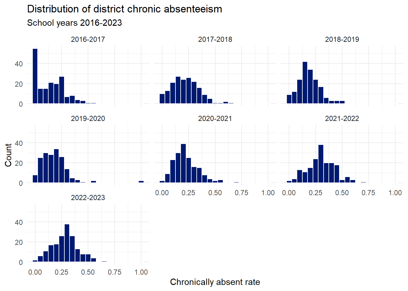
df_master |>ggplot(aes(x=chronically_absent_rate)) +geom_histogram(binwidth =0.05, colour="white", fill=standard_chart_colour) +facet_wrap(~school_year) +labs(title ="Distribution of district chronic absenteeism",subtitle ="School years 2016-2023",x="Chronically absent rate",y="Count" )
The data look valid. There is a high occurrence of zero values in the 2016-2017 school year. This suggests that either different school districts may have begun record keeping at different times or that these smaller districts were actually not seeing this phenomenon until later. Of these, the former seems more plausible. Chronic absenteeism could be cross-referenced with truancy rates to provide a check on this. The truancy data may allow us to rule out the second hypothesis. This could be done in a follow-up analysis.
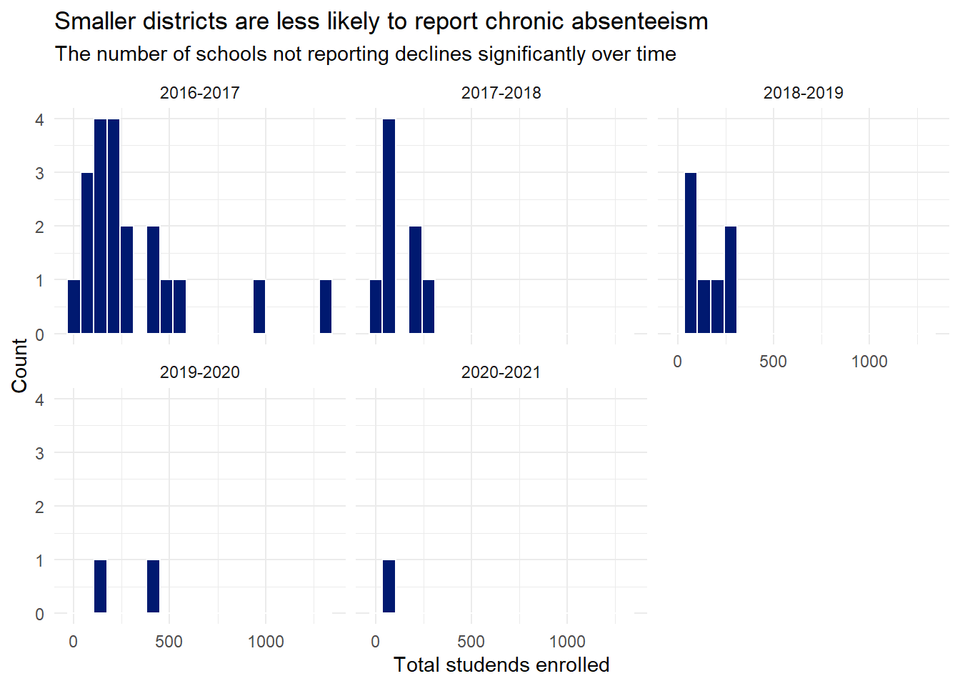
There are 20 districts that reported no chronically absent students in 2016-2017. The number steadily decreases and by 2021-2022 there are no districts reporting no students as chronically absent.
df_master |>filter(chronically_absent_rate ==0) |>ggplot(aes(x=total_students)) +geom_histogram(bins=20, colour="white", fill=standard_chart_colour) +facet_wrap(~school_year) +labs(title ="Smaller districts are less likely to report chronic absenteeism",subtitle ="The number of schools not reporting declines significantly over time",x="Total studends enrolled",y="Count" )
Total student enrollment
Based on a 5-number summary of the number of students enrolled in each district varies widely from less than 10 to more than 85,000.
5-number summary of undifferentiated enrollment data
school_year
min_count
quartile_1
median
quartile_3
max_count
2016-2017
5
212
596
2,339
86,139
2017-2018
4
210.5
584
2,325.5
86,863
2018-2019
37
209
598
2,299
86,887
2019-2020
16
227.2
658.5
2,475.2
96,030
2020-2021
44
219
622
2,193
93,385
2021-2022
32
225.5
619.5
2,369.8
92,170
2022-2023
31
222
599
2,322
87,225
The numbers are consistent and there are no obviously invalid values in the dataset. The minimum counts for the first two years look suspect. The district is the same in both cases, the Agate 300 school district.
df_master |>filter(district_code =="0960") |>select(school_year,absentee_students,total_students,chronically_absent_rate) |>gt(id="agate-300-enrollment") |>format_table("Agate 300 School District enrollment data 2016-2023")
Agate 300 School District enrollment data 2016-2023
school_year
absentee_students
total_students
chronically_absent_rate
2016-2017
0
5
0
2017-2018
0
4
0
2018-2019
0
47
0
2019-2020
4
34
0.1
2020-2021
16
73
0.2
2021-2022
22
95
0.2
2022-2023
12
78
0.2
The total_students data for Agate 300 school district is quite variable, but 5 and 4 seem like extremely low counts given the other 5 years of data available. It will not affect the outcome of this study, but a follow-up to determine the true values for the 2016-2017 and 2017-2018 school years would be useful.
To look for more school districts that might have large discrepancies in enrollment, year on year percent change in total enrollment can be computed and outliers investigated. After the field is created, a 5-number summary will give rough information about how the values are distributed.
% change in enrollment 5-number summary by school year
school_year
min_diff
quartile_1
median
quartile_3
max_diff
2017-2018
−24.1
−2.4
0.1
2.2
47.1
2018-2019
−16.9
−2.1
0.2
2.5
1,075
2019-2020
−90.4
4.7
9.6
14.7
75.6
2020-2021
−81
−8.9
−3.9
0
868.8
2021-2022
−66.3
−3.4
1.5
7.2
395.5
2022-2023
−46.6
−9
−4.3
−0.2
217.8
This table shows that there are some very significant changes in district enrollments.
df_master_tmp |>filter(school_year !="2016-2017"&abs(pct_enroll_diff) >50) |>select(school_year, district_code, district_name, absentee_students, total_students, pct_enroll_diff) |>arrange(desc(abs(pct_enroll_diff))) |>gt(id="colorado-pct-diff-enrollment") |>format_table("Percent change of enrollment outliers 2016-2023","Outliers are defined as having a change in enrollment greater than 50%")
Percent change of enrollment outliers 2016-2023
Outliers are defined as having a change in enrollment greater than 50%
school_year
district_code
district_name
absentee_students
total_students
pct_enroll_diff
2018-2019
0960
Agate 300
0
47
1,075
2020-2021
1410
North Park R-1
35
155
868.8
2021-2022
0100
Alamosa Re-11j
685
2,294
395.5
2020-2021
0230
Walsh Re-1
31
160
255.6
2022-2023
1440
Plainview Re-2
6
410
217.8
2020-2021
0260
Vilas Re-5
6
200
177.8
2022-2023
0310
McClave Re-2
42
236
168.2
2021-2022
1440
Plainview Re-2
12
129
158
2021-2022
0940
Big Sandy 100j
56
354
139.2
2020-2021
3220
Idalia Rj-3
21
185
134.2
2020-2021
0960
Agate 300
16
73
114.7
2021-2022
0740
Sierra Grande R-30
87
286
110.3
2020-2021
1590
Primero Reorganized 2
29
223
106.5
2021-2022
0580
South Conejos Re-10
32
155
98.7
2019-2020
1410
North Park R-1
2
16
−90.4
2021-2022
3110
Johnstown-Milliken Re-5j
947
3,906
83.5
2020-2021
0100
Alamosa Re-11j
127
463
−81
2021-2022
2862
Julesburg Re-1
328
742
80.5
2019-2020
0260
Vilas Re-5
12
72
75.6
2020-2021
0190
Byers 32j
2,115
7,027
73.5
2019-2020
0230
Walsh Re-1
3
45
−69.8
2021-2022
0290
Las Animas Re-1
350
859
−66.3
2022-2023
1580
Trinidad 1
238
856
64.6
2021-2022
0310
McClave Re-2
13
88
−59.8
2019-2020
3220
Idalia Rj-3
79
79
−57.8
2020-2021
1440
Plainview Re-2
10
50
56.2
2019-2020
2862
Julesburg Re-1
167
802
55.4
2019-2020
0170
Deer Trail 26j
61
283
53.8
2020-2021
0580
South Conejos Re-10
11
78
−51.2
Without knowing the history if these districts it is hard to say if the numbers contain errors. Like Agate 300, mentioned earlier, there are some very large changes year on year in micro to intermediate sized districts. Some of this may be explained by small districts be subject to more size volatility than larger ones, but some of these districts are having order of magnitude size changes in total enrollment which seems likely to be a data entry error than a real fluctuation in student enrollment.
Examples of districts with at least 1 suspicious total_students record
0960 - Agate 300
0230 - Walsh RE-1
1410 - North Park R-1
0100 - Alamosa Re-11j
0580 - South Conejos Re-10 (?)
The first two years for Agate show enrollments of 5 & 4 students, then enrollment jumps to 37. It is likely that the 5 and 4 should be 35 and 34, but without checking, it is hard to say what the correct values are.
For Walsh RE-1, there is a clear typo in the 2019-2020 information. The listed value is 45 but this should probably be 145 based on the other years.
The same situation exists for North Park R-1 and in the same year. The listed value is 16, but it should probably be 160 or similar based on data from the other school years.
Alamosa RE-11j has a similar issue in the 2020-2021 school year where, most likely, a leading “2” was dropped from the total enrollment number. It should probably be 2463 rather than the 463 that is listed.
There is a less clear case for the South Conejos Re-10 school district in 2021-2022. The total enrollment drops from 160 to 78 before rebounding to 155. It is possible that there is a leading “1” that is missing, but so many districts show a drop in this year, that it is possible that the data are accurate.
Chronically absent student counts
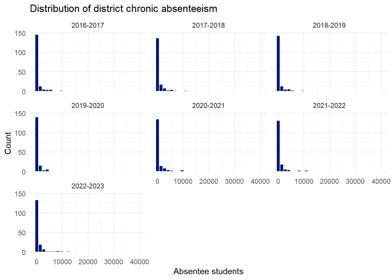
The number of chronically absent students in each district varies widely from 0 to more than 40,000. The numbers are consistent and there are no invalid values in the dataset.
df_master |>filter(!is.na(absentee_students)) |>ggplot(aes(x=absentee_students)) +geom_histogram(colour="white", fill=standard_chart_colour) +facet_wrap(~school_year) +labs(title ="Distribution of district chronic absenteeism",x="Absentee students",y="Count" )
Feature creation
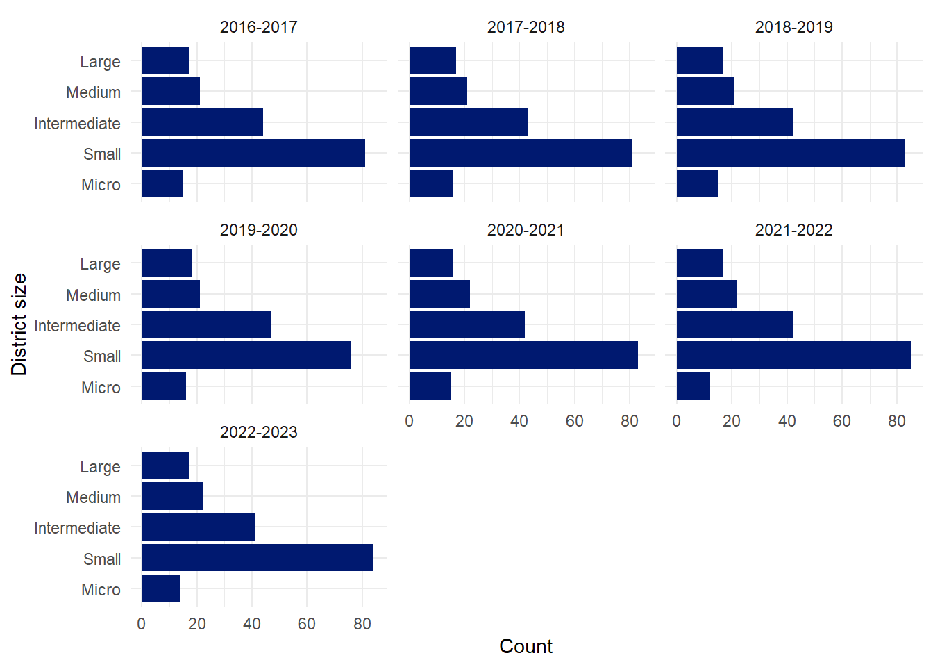
Three new features will be made from the current data: district_size, pct_diff, and pct_enrollment_diff. The first feature is a ordered categorical variable that describes the size of the district. There are five levels. From smallest to largest they are
Micro - Up to 100 students
Small - 101 to 750 students
Intermediate - 751 to 3000 students
Medium - 3001 to 15000 students
Large - More than 15000 students
The second feature is the change in chronic absenteeism rate from year to year. The values for all districts in the 2016-2017 school year are NA as this is the first year in the dataset.
The number of districts in each group is consistent from year to year. The smaller school districts, those in the Small and Micro categories, have the most variability. This is not surprising as small changes in student population can move a district from one category to another.
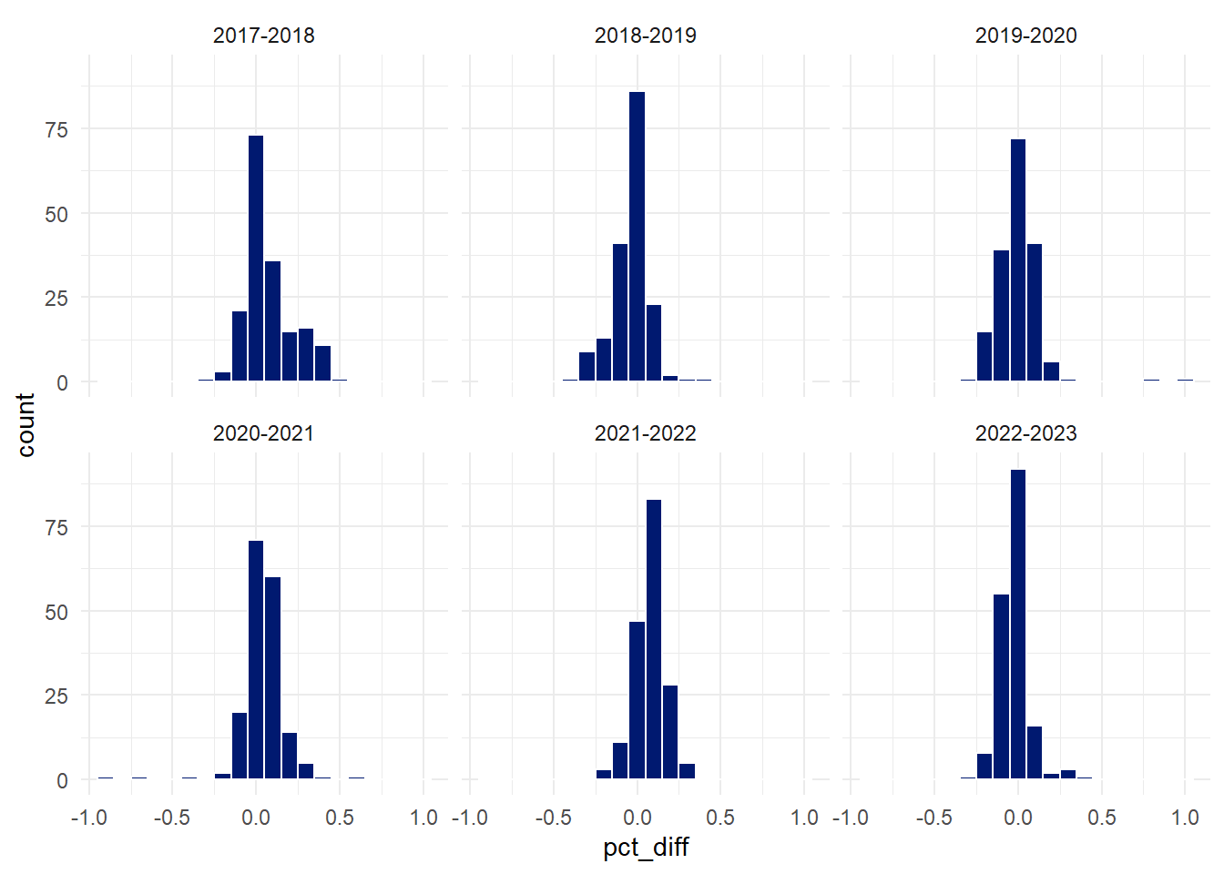
The pct_diff data looks to be consistent with what we know about the rest of the data in this dataset. The 5 number summary shows how volatile the absenteeism rates can be, particularly around the first COVID-19 school year 2019-2020.